Random variables

Informally, random variables are real-valued functions on probability spaces. Such functions induce probability measures on $\mathbb{R}$, which encompass all of the familiar probability distributions. These distributions are, essentially, probability measures on the set of real numbers; to formalize this, we need to be able to articulate probability spaces with $\mathbb{R}$ as the sample space.

The Borel sets comprise the smallest $\sigma$-algebra containing all intervals contained in $\mathbb{R}$. We will denote this collection by $\mathcal{B}$; while it is possible to generate $\mathcal{B}$ constructively from the open intervals as a closure under complements, countable unions, and countable intersections, doing so rigorously is beyond the scope of this class. Importantly, however, $\mathcal{B}$ contains all intervals and all sets that can be formed from intervals; these will comprise our “events” of interest going forward.

Concepts

Let $(S,\mathcal{S},P)$ be a probability space. A random variable is a function $X:S⟶\mathbb{R}$ such that for every $B\in \mathcal{B}$, $X^{-1}(B)\in \mathcal{S}$.

Example: coin toss

If $S=\{H,T\}$, and $\mathcal{S}=2^S=\{\mathrm{\varnothing },\{H\},\{T\},\{H,T\}\}$, define: $$X(s)=\{\begin{array}{ll}1,& s=H\\ 0,& s\ne H\end{array}$$ Then $X$ is a random variable since for any $B\in \mathcal{B}$: $$X^{-1}(B)=\{\begin{array}{ll}\{H\},& 1\in B\\ \{T\},& 0\in B\end{array}$$ So $X^{-1}(B)\in \mathcal{S}$.

Not all functions are random variables. For example, take $S=\{1,2,3\}$ and the trivial $\sigma$-algebra $\mathcal{S}=\{\mathrm{\varnothing },S\}$, and consider $X(s)=s$; then $X^{-1}(2)=2\notin \mathcal{S}$.

The condition that preimages of Borel sets be events ensures that we can associate probabilities to statements such as $a<X(s)<b$ or, more generally $X\in B$. Specifically, we can assign such statements probabilities according to the outcomes in the underlying probability space that map to $B$ under $X$. Thus, random variables induce probability measures on $\mathbb{R}$.

More precisely, if $(S,\mathcal{S},P)$ is a probability space and $X:S⟶\mathbb{R}$ is a random variable, then the induced probability measure (on $\mathbb{R}$) is defined for any Borel set $B\in \mathcal{B}$ as: $$P_X(B)=P(X^{-1}(B))$$

The induced measure $P_X$ is known more commonly as a probability distribution or simply as a distribution: it describes how probabilities are distributed across the set of real numbers.

Example

You’ve already seen some simple random variables. For example, on the probability space representing two dice rolls with all outcomes equally likely, that is, $S=\{1,\dots ,6{\}}^2$ with $\mathcal{S}=2^S$ and $P(E)=\frac{|E|}{36}$, the function $X((i,j))=i+j$ is a random variable, because $X^{-1}(B)=\{(i,j):i+j=x\text{ for some }x\in B\}\in 2^S$. Moreover, the probability distribution associated with $X$ is:

$$P_X(B)=\frac{1}{36}\sum _{x\in B}|\{(i,j)\in S:i+j=x\}|$$ As determined in a previous homework problem, $|\{(i,j)\in S:i+j=x\}|>0$ only for $x=2,3,\dots ,12$, and the associated probabilities are:

x	$P_X(\{x\})$
2	$\frac{1}{36}$
3	$\frac{2}{36}$
4	$\frac{3}{36}$
5	$\frac{4}{36}$
6	$\frac{5}{36}$
7	$\frac{6}{36}$
8	$\frac{5}{36}$
9	$\frac{4}{36}$
10	$\frac{3}{36}$
11	$\frac{2}{36}$
12	$\frac{1}{36}$

Cumulative distribution functions

We must remember that the concept of a distribution arises relative to some underlying probability space. However, it is not necessary to work with the underlying measure — distributions, luckily, can be characterized using any of several real-valued functions. Arguably, the most fundamental of these is the cumulative distribution function (CDF).

Given any random variable $X:S⟶\mathbb{R}$, define the cumulative distribution function (CDF) of $X$ to be the function: $$F_X(x)=P_X((-\mathrm{\infty },x])=P(\{s\in S:X(s)\le x\})$$

Check your understanding

Consider the dice roll example above with the random variable $X((i,j))=i+j$. Fill in the table below, and then draw the CDF.

x	$P_X(\{x\})$	$P(X\le x)$
2	$\frac{1}{36}$
3	$\frac{2}{36}$
4	$\frac{3}{36}$
5	$\frac{4}{36}$
6	$\frac{5}{36}$
7	$\frac{6}{36}$
8	$\frac{5}{36}$
9	$\frac{4}{36}$
10	$\frac{3}{36}$
11	$\frac{2}{36}$
12	$\frac{1}{36}$

If the random variable is evident from context, the subscript can be omitted and one can write $F$ instead of $F_X$.

Theorem. $F$ is the CDF of a random variable if and only if it satisfies the following four properties:

1. $\underset{x\to -\mathrm{\infty }}{lim}F(x)=0$
2. $\underset{x\to \mathrm{\infty }}{lim}F(x)=1$
3. $F$ is monotone nondecreasing: $x\le y\Rightarrow F(x)\le F(y)$
4. $F$ is right-continuous: $\underset{x\downarrow x_0}{lim}F(x)=F(x_0)$

Proof

We will prove the ‘necessity’ part: that if a random variable has CDF $X$, then it satisfies (i)-(iv) above. For sufficiency, one must construct a probability space and random variable $X$ such that $X$ has CDF $F$; we will skip this argument, as it is beyond the scope of this class.

For (i), observe that $E_n=\{s\in S:X(s)\le -n\}$ is a nonincreasing sequence of sets for $n\in \mathbb{N}$ and $\underset{n}{lim}{E}_n=\bigcap _n{E}_n=\mathrm{\varnothing }$. Then: $$\underset{x\to -\mathrm{\infty }}{lim}F(x)=\underset{n\to \mathrm{\infty }}{lim}F(-n)=\underset{n\to \mathrm{\infty }}{lim}P(E_n)=P\left(\underset{n\to \mathrm{\infty }}{lim}{E}_n\right)=0$$

For (ii), observe that $E_n=\{s\in S:X(s)\le n\}$ is a nondecreasing sequence of sets for $n\in \mathbb{N}$ and $\underset{n}{lim}{E}_n=\bigcup _n{E}_n=S$. Then: $$\underset{x\to \mathrm{\infty }}{lim}F(x)=\underset{n\to \mathrm{\infty }}{lim}F(n)=\underset{n\to \mathrm{\infty }}{lim}P(E_n)=P\left(\underset{n\to \mathrm{\infty }}{lim}{E}_n\right)=1$$ For (iii), note that if $x\le y$ then $\{s\in S:X(s)\le x\}\subseteq \{s\in S:X(S)\le y\}$, so by monotonicity of probability $F(x)\le F(y)$.

For (iv), let $\{x_n\}$ be any decreasing sequence with $x_n\to x_0$. For instance, $x_n=x_0+\frac{1}{n}$. Then the sequence of events $E_n=\{s\in S:X(s)\le x_n\}$ is nonincreasing, and $\underset{n}{lim}{E}_n=\bigcap _n{E}_n=\{x\in S:X(s)\le x_0\}$, so: $$\begin{array}{rl}\underset{x\downarrow x_0}{lim}F(x)& =\underset{n\to \mathrm{\infty }}{lim}F(x_n)\\ & =\underset{n\to \mathrm{\infty }}{lim}P(E_n)\\ & =P\left(\underset{n\to \mathrm{\infty }}{lim}{E}_n\right)\\ & =P(\{x\in S:X(s)\le x_0\})\\ & =F(x_0)\end{array}$$

The portion of this theorem we didn’t prove is perhaps the more consequential part of the result, as it establishes that if $F$ is any function satisfying properties (i)–(iv) then there exists a probability space and random variable $X$ such that $F_X=F$. This means that we can omit reference to the underlying probability space $(S,\mathcal{S},P)$ since some such space exists for any CDF. Thus, we will write probabilities simply as, e.g., $P(X\le x)$ in place of $P_X((-\mathrm{\infty },x])$ or $P(\{s\in S:X(s)\le x\})$. Consistent with this change in notation, we will speak directly about probability distributions as distributions “of” (rather than “induced by”) random variables.

It’s important to remember that distributions and random variables are distinct concepts: distributions are probability measures ($P_X$ above) and random variables are real-valued functions. Many random variables might have the same distribution, yet be distinct. Since CDFs are one class of functions that uniquely identify distributions, if two random variables $X,Y$ have the same CDF (that is if $F_X=F_Y$) then they have the same distribution and we write $X\stackrel{d}{=}Y$

Two convenient properties of CDFs are:

• If $X$ is a random variable with CDF $F$, then $P(a<X\le b)=F(b)-F(a)$
• If $X$ is a random variable with CDF $F$, then $P(X>a)=1-F(a)$

The proofs will be left as exercises. This section closes with a technical result that characterizes the probabilities of individual points $x\in \mathbb{R}$.

Lemma. Let $X$ be a random variable with CDF $F$. Then $P(X=x)=F(x)-F(x^{-})$, where $F(x^{-})$ denotes the left-hand limit $\underset{z\uparrow x}{lim}F(z)$.

Proof

Define $E_n=\{x-\frac{1}{n}<X\le x\}$; then $P(E_n)=F(x)-F(x-\frac{1}{n})$ and $\{E_n\}$ is a nonincreasing sequence with $\underset{n}{lim}{E}_n=\{X=x\}$. Then: $$\begin{array}{rl}P(X=x)& =P(\underset{n\to \mathrm{\infty }}{lim}{E}_n)\\ & =\underset{n\to \mathrm{\infty }}{lim}P(E_n)\\ & =\underset{n\to \mathrm{\infty }}{lim}[F(x)-F(x-\frac{1}{n})]\\ & =F(x)-\underset{n\to \mathrm{\infty }}{lim}F(x-\frac{1}{n})\\ & =F(x)-\underset{z\uparrow x}{lim}F(x)\\ & =F(x)-F(x^{-})\end{array}$$

Notice the implication that if $F$ is continuous everywhere, then $P(X=x)=0$ for every $x\in \mathbb{R}$.

Discrete random variables

If a CDF takes on countably many values, then the corresponding random variable is said to be discrete. For discrete random variables, $P(x=x)$ is called the probability mass function (PMF) and the probability of any event $E\in \mathcal{B}$ is given by the summation: $$P_X(E)=P(X\in E)=\sum _{x\in E}P(X=x)$$

It can be shown that discrete random variables take countably many values — i.e., $P(X=x)>0$ for countably many $x\in \mathbb{R}$. We call the set of points where the probability mass function is positive — $\{x\in \mathbb{R}:P(X=x)>0\}$ — the support set (or simply the support) of $X$ (or its distribution).

Theorem. A function $f$ is the PMF of a discrete random variable if and only if:

1. $0\le f(x)\le 1$
2. $\sum _{x\in \mathbb{R}}f(x)=1$

Proof

If $f$ is a PMF of a discrete random variable $X$, then by definition the PMF is $f(x)=F(x)-F(x^{-})$. Since $F(x)\le F(x^{-})$ by monotonicity of $F$, $f(x)\ge 0$ for every $x$. Since $\underset{x\to \mathrm{\infty }}{lim}F(x)=1$ and $F$ is monotonic, $F(x)\le 1$ for every $x$; by construction $f(x)\le F(x)\le 1$. So $0\le f(x)\le 1$.

For the converse implication, if $f$ is a function satisfying (i)–(ii), then $f(x)>0$ for only countably many values. To see this, consider $A_n=\{x\in \mathbb{R}:\frac{1}{n+1}\le f(x)<\frac{1}{n}\}$ for $n=1,2,\dots$ with $A_0=\{x\in \mathbb{R}:f(x)=1\}$; by construction we must have $\sum _{x\in \mathbb{R}}f(x)\ge \sum _{x\in A_n}f(x)$ for every $n$ since $f$ is nonnegative per (i) and $A_n\subseteq \mathbb{R}$. Now $f(x)\ge \frac{1}{n+1}$ on $A_n$ so $\sum _{x\in A_n}f(x)\ge \sum _{x\in A_n}\frac{1}{n+1}$; but then if $A_n$ is infinite the sum on the right diverges, and thus so does the sum over all $x\in \mathbb{R}$ contrary to (ii). So (ii) entails that $|A_n|<\mathrm{\infty }$ for every $n$, and thus the union $\bigcup _{n=1}{A}_n=\{x\in \mathbb{R}:f(x)>0\}$ is a countable set.

Let $S$ denote the set $\{x\in \mathbb{R}:f(x)>0\}$. Let $x_1,x_2,\dots$ denote the elements of $S$ and $p_1,p_2,\dots$ denote the corresponding values of $f$, that is, $p_i=f(x_i)$. By hypothesis we have that $0\le p_i\le 1$ (condition (i)) and $\sum _{i=1}^{\mathrm{\infty }}{p}_i=1$ (condition (ii)). Let $P(E)=\sum _{i:x_i\in E}{p}_i$ for $E\in 2^S$. Then $P$ is a probability measure on $(S,2^S)$ — it suffices to check that $P$ satisfies the probability axioms.

• Axiom 1: $P(E)=\sum _{i:x_i\in E}{p}_i\ge 0$ since by hypothesis $p_i\ge 0$.
• Axiom 2: $P(S)=\sum _{i:x_i\in S}{p}_i=\sum _{i=1}^{\mathrm{\infty }}{p}_i=1$.
• Axiom 3: let $\{E_j\}$ be disjoint and define $I_j=\{i:x_i\in E_j\}$. Note that $\{i:x_i\in \bigcup _j{E}_j\}=\bigcup _j{I}_j$ and $I_j\cap I_k=\mathrm{\varnothing }$ for $j\ne k$. Then: $P\left(\bigcup _j{E}_j\right)=\sum _{\bigcup _j{I}_j}{p}_i=\sum _j\sum _{I_j}{p}_i=\sum _{j}P(E_j)$

So $(S,2^S,P)$ is a probability space. Now let $X$ be the identity map $X(s)=s$. $X$ is a random variable, since $X^{-1}(B)=\{x_j{\}}_{j\in J}\in 2^S$ for every $B\in \mathcal{B}$, and its CDF is given by $F(x)=\sum _{\{i:x_i\le x\}}{p}_i$. This is a step function with countably many values, so $X$ is a discrete random variable. Finally, it is easy to check that:

$$P(X=x)=F(x)-F(x^{-})=\{\begin{array}{ll}0& x\notin S\\ p_i& x=x_i\end{array}$$

So $X$ has PMF $P(X=x_i)=p_i=f(x_i)$ as required.

This result shows that PMFs uniquely determine discrete distributions. It also establishes that the support set is countable, so the unique values can be enumerated as $\{x_1,x_2,\dots ,x_i,\dots \}$. We can recover the CDF from the PMF as $F(x)=\sum _{x_i\le x}P(X=x_i)$.

Continuous random variables

If a CDF is absolutely continuous everywhere then the corresponding random variable is said to be continuous. In this case, $P(X=x)=0$ for every $x\in \mathbb{R}$ and so we define instead the probability density function (PDF) to be the function $f$ such that $$F(x)={\int }_{-\mathrm{\infty }}^{x}f(z)dz$$

By the fundamental theorem of calculus, one has that $f(x)=\frac{d}{dx}F(x)$. The probability of any event $E\in \mathcal{B}$ is given by the integral: $$P_X(E)=P(X\in E)={\int }_{E}f(x)dx$$

For continuous random variables, the support set is defined as the set of points with positive density, that is, $\{x\in \mathbb{R}:f(x)>0\}$.

Similar to the theorem above for discrete distributions, it can be shown that a function $f$ is the PDF of a continuous random variable if and only if:

1. $f(x)\ge 0$
2. ${\int }_{\mathbb{R}}f(x)dx=1$

The proof of this result is omitted.

Exercise: characterizing distributions

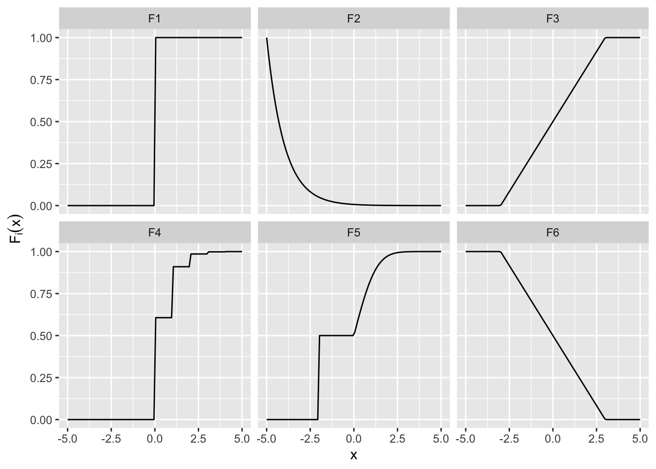
For each of the functions below, determine whether it is a CDF. Then, for the CDFs, identify whether a random variable with this distribution is discrete or continuous, and find or guesstimate the PMF/PDF if it exists. You can ignore the behavior at the endpoints, but to check your understanding, identify for each jump which value the function must take at the endpoint for it to be a valid CDF.

These results establish that all distributions (again, recall that technically distributions are probability measures on $\mathbb{R}$ induced by random variables) can be characterized by CDFs or PDF/PMFs. If a random variable $X$ has the distribution given by the CDF $F$ or the PDF/PMF $f$, we write

$$X\sim F(x)\text{or}X\sim f(x)$$

respectively.